Similar to Random Forests, Extreme Gradient Boosting, or XGBoost, uses a string of decision trees in order to help make predictions. However, while RF models use bagging, selecting the most commonly chosen answer to be the best one overall, Boosting models like XGBoost, building new models sequentially in order to minimize the errors of both old and new attempts.
The code to import xg boost from the SKLearn library is as follows:

from xgboost.sklearn import XGBClassifier

This sequential approach works in a small series of steps:

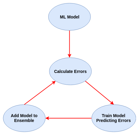
Individual tests are not strong enough to make an accurate predictions, they are called weak learners. A weak learner acts as a classifier that has less of a correlation with the actual value. Therefore, to make our predictions more accurate, we devise a model that combines weak learners’ predictions to make a strong learner, and this is done using the technique of boosting. Since XGBoost uses Decision Trees as its weak learners, we can say that it is a Tree based learner.

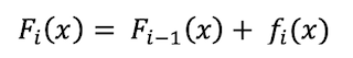
We fist fit a first weak model using the original data, creating a single decision tree as a predictor. Then we create a residual model (prediction), proceeding to correct that model using a gradient descent algorithm to minimize a loss function, which should show a positive increase in performance from model to model. Loss normally means the difference between the predicted value and actual value. Based off of that loss function a new model is created from the sum of models 1 and 2 as follows. Capital F(i) represents the current model, F(i-1) is the previous model and small f(i) represents a weak model.

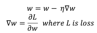
For gradient boosting specifically, we use an algorithm called Gradient Descent, which iteratively optimizes the loss of the model by updating the weights of features. For classification problems, we use logarithmic loss calculations to make these predictions. In this case, w represents the weight vector, η is the learning rate

If you want to learn more about Gradient Boosting, and what makes XGBoost's implementation so efficient, click the link here:

XGBoost: A Deep Dive into Boosting

Our XGBoost Experience

Data and Analysis

We found that XGBoost was our most accurate and reliable algorithm to use across multiple trials due to its high recall, precision and accuracy scores. All of our scores were high, but XGBoost was the most consistent, having the lowest error rate across multiple trials. This was especially apparent on the heat maps produced for the results of these trails (an example of which is pictured below).

Accuracy Score

Precision Score

Recall

ROC AUC Score

Hyperparameter Tuning

learning_rate

In each boosting step, this values shrinks the weight of new features, preventing overfitting or a local minimum. This value must be between 0 and 1. The default value is 0.3. - We set our learning rate to be 0.1

max_depth

The maximum depth of a tree. The greater the depth, greater the complexity of the model and more easy to overfit. This value must be an integer greater than 0 and have 6 as default - we kept it at 6.

n_estimators

The number of trees in our ensemble. - set to be default (100)

colsample_bytree

Represents the fraction of columns to be subsampled. It’s related to the speed of the algorithm and prevent overfitting. Default value is 1 but it can be any number between 0 and 1. - We set it to 0.7

gamma

A regularization term and it’s related to the complexity of the model. It’s the minimum loss necessary to occur a split in a leaf. It can be any value greater than zero and has a default value of 0.